6 MBL Models
This section of the demo script creates MBL models and gets predictions from them:
#----------------------------------------------#
# Memory Based Learner Model #
#----------------------------------------------#
source("Functions/mbl_functions.R")
source("Functions/perform_functions.R")

# Make Model
mbl.OC <- runMBL(PROP="OC", REFNAME="refSet", PREDNAME="predSet")

# Extract Predictions
mbl.predictions <- getModResults(PROP="OC", MODTYPE="MBL", MODNAME= "mbl.OC", PREDNAME= "predSet")
Model Theory
Overview
Memory-Based Learning (MBL) is a local modeling approach that can be used to predict a given soil property from a set of spectral data, the prediction set.
Like PLS, this approach relies on a reference set, containing both spectral data and known values for the soil property of interest (ie. Organic Carbon).
While PLS create a single global model which can be applied to all samples in the prediction set, MBL makes a local model for each prediction.
Local models are built from a sample’s nearest neighbors: samples in the reference set that are most similar to the sample being predicted.
Similarity is measured by spectral similarity, which should reflect similarities in soil composition. Since each sample has a customized model, predictions are often more accurate than PLS predictions.
However, MBL models can be quite computationally intensive since
1) A model is built for each sample being predicted
2) All samples in the prediction and reference set must be related in terms of similarity
Animation
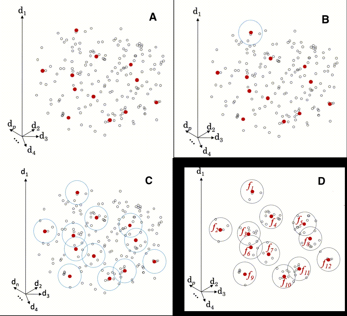
The animation below illustrates how local modeling works in MBL. It is shown in multidimensional space since each spectral column is a dimension of the dataset.

A Shows all the samples in the prediction set (red), overlaying all the samples in the reference set (gray)
B Shows a circle indicating the nearest neighbors of a sample being predicted
C Shows all the samples of the prediction set with their respective nearest neighbors
D Shows how local models will be created for each prediction from these nearest neighbors
Resemble Powerpoint: http://www.fao.org/fileadmin/user_upload/GSP/docs/Spectroscopy_dec13/SSW2013_f.pdf
Running MBL
Running an MBL modeling approach is accomplished using a couple functions from the resemble package: mblControl() and mbl(). Full documentation for these functions is linked below and the following sections describe how they can be used.
MBL- Resemble mbl() Documentation
mbl(Yr, Xr, Yu = NULL, Xu,
    mblCtrl = mblControl(),
    dissimilarityM,
    group = NULL,
    dissUsage = "predictors",
    k, k.diss, k.range,
    method,
    pls.c, pls.max.iter = 1, pls.tol = 1e-6,
    noise.v = 0.001,
    ...)
MBL Control- Resemble mblControl() Documentation
mblControl(sm = "pc",
           pcSelection = list("opc", 40),
           pcMethod = "svd",
           ws = if(sm == "movcor") 41,
           k0,
           returnDiss = FALSE,
           center = TRUE,
           scaled = TRUE,
           valMethod = c("NNv", "loc_crossval"),
           localOptimization = TRUE,
           resampling = 10,
           p = 0.75,
           range.pred.lim = TRUE,
           progress = TRUE,
           cores = 1,
           allowParallel = TRUE)
runMBL()
runMBL() is a wrapper function for loading the appropriate datasets and calling the resemble functions for running an mbl model. It is used directly in the demo script as shown below:
source("Functions/mbl_functions.R")
mbl.OC <- runMBL(PROP="OC", REFNAME="refSet", PREDNAME="predSet")runMBL()PROP: string- The column name of the soil property of interest.REFNAME: string- The name of the reference set variable, if it is already loaded into the R environment. Use REFNAME or REFPATHREFPATH: string- The path of the RData file containing your reference set, if the reference set is not already loaded. Use REFNAME or REFPATHPREDNAME: string- The name of the prediction set variable, if it is already loaded into the R environment. Use PREDNAME or PREDPATHPREDPATH: string- The path of the RData file containing your prediction set, if the prediction set is not already loaded. Use PREDNAME or PREDPATHSAVENAME: string- The name assigned to the model when it is saved. Default is set to paste0(“mbl.”,PROP) which would save “mbl.OC.RData” for example in the “Models” folder
_
- Load the resemble package
- Load the data
- If
REFPATHis not NA, it will load the reference set at the path passed. Otherwise, it assumes you have passed inREFNAME, the variable name of a reference set already loaded. We use theget()command, rather than the variable itself, so that the name of the variable can be saved with our prediction performance. The same applies to the prediction set.
- If
# Load Reference Set
if(!is.na(REFPATH)){
  REFNAME <- load(REFPATH) # If REFPATH is given
}
refset <- get(REFNAME) # load as variable REFSET

# Load Prediction Set
if(!is.na(PREDPATH)){
  PREDNAME <- load(PREDPATH)
}
predSet <- get(PREDNAME)- Define inputs and eliminate rows with NA values
# Define Input Datasets
Xu <- predSet$spc          # Prediction Spectra
Yu <- sqrt(predSet[,PROP]) # Prediction Lab Data
Yr <- sqrt(refSet[,PROP])  # Reference Spectra
Xr <- refSet$spc           # Reference Lab Data

# Get Rid of NAs
Xu <- Xu[!is.na(Yu),]
Xr <- Xr[!is.na(Yr),]
Yu <- Yu[!is.na(Yu)]
Yr <- Yr[!is.na(Yr)]- Set Control Parameters
- In this example, nearest neighbors will be determined in principal component space (
sm='pc'), the optimal number of principal components will be used and up to 50 components will be tested (pcSelection = list('opc',50)), and nearest neighbor validation will be used (valMethod = 'NNv')- meaning for each prediction, a model will be built will all but the nearest neighbor of the sample being predicted.
- In this example, nearest neighbors will be determined in principal component space (
ctrl <- mblControl(sm = 'pc', pcSelection = list('opc', 50),
valMethod = 'NNv',center=TRUE,scale=FALSE,allowParallel=FALSE)- Run MBL Model
- Option 1 - Will make local partial least squares regression models using 40, 60, 80 and 100 nearest neighbors (
k= seq(40, 100, by = 20)) and using 6 components (pls.c = 6) to make predictions. Will not use the dissimilarity matrx (dissUsage = 'none'). - Option 2- Will create weighted partial least squares regression models (
method = "wapls1") using the neighbors within 0.3, 0.4,…1 distance from the sample being predicted (k.diss = seq(0.3, 1, by=0.1)), with a minimum of 20 neighbors used (k.range = c(20, nrow(refSet))) and predicting with 3 to 20 of the components of the model (pls.c = c(minpls=3, maxpls=20))
- Option 1 - Will make local partial least squares regression models using 40, 60, 80 and 100 nearest neighbors (
Option 1
  mbl.sqrt <- mbl(Yr = Yr, Xr = Xr, Yu = Yu, Xu = Xu, mblCtrl = ctrl, dissUsage = 'none',
                  k = seq(40, 100, by = 20), method = 'pls', pls.c = 6)
Option 2
mbl.sqrt <- mbl(Yr = Yr, Xr = Xr, Xu = Xu, mblCtrl = ctrl, dissUsage = "none", k.diss = seq(0.3, 1, by=0.1),
k.range = c(20, nrow(refSet)), pls.c = c(minpls=3, maxpls=20), method = "wapls1")- Save the model
# Save MBL Model
if(SAVENAME != "none"){
  modelName <- paste("mbl", PROP, sep=".") # Assign Object Name
  assign(modelName, mbl.sqrt)
  savefile <- paste("./Models/mbl", PROP,"RData", sep=".") # Save File
  save(list= modelName, file = savefile)
  cat(paste("\nModel",modelName, "saved to", savefile)) # Print Save Location
}
Modeling Parameters
This section explains some of the main ways to customize and optimize mbl models using mbl() and mblControl() in the resemble package. Full documentation on these functions are linked below:
Below is an example workflow showing the decision points of modeling with MBL. These parameters will be describe in the following subsections.

Input Datasets
- The
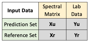
mbl()function accepts 4 different data products,XuXrYuandYr, summarized in the table below:

- Both Xs are matrices with spectral data and both Ys are vectors with lab data for the property of interest.
- u indicates “uncertain” for our prediction set, and r indicates “reference” for our reference set.
Yuis optional, since not all prediction sets will have associated lab data. If this is the case, setYutoNULL.- See the data preprocessing tab to prepare these datasets prior to modeling. In addition, it is necessary to remove all rows in the reference set inputs (
YrandXr) that haveNAvalues. If you would like to includeYubut there are missing values, you must also remove those rows in both prediction set inputs (YuandXu).- Number of columns in
Xrmust equal that ofXu. - Number of rows in
Yrmust equal that ofYu, if provided.
- Number of columns in
Matrix of Spectral Neighbors
When selecting nearest neighbors to build a local model, the
mbl()function references a spectral dissimilarity matrix, which relates samples in the prediction and reference sets.This matrix can be created by setting the
smparameter inmblControl(), or can be passed into thembl()function asdissimilarityMif a matrix has already been made.- For creating the matrix, you will have to decide how spectral dissimilarity will be calculated by setting a couple variables in mblControl():
smcan be set to a variety of different methods for measuring distance in a multidimensional space. We have used"pls" "pc" "euclid" "cosine" "cor" and "movcor"pcSelectiondetermines how the number of principal components will be chosen for calculating Mahalonobis dissimilarity (when sm = “pc”, “loc.pc”, “pls” or “loc.pls”)- We have this set to the default options of
(opc,40)meaning the optimal principal component method will be used and up to 40 components will be tested.
.
- We have this set to the default options of
- Lastly, you can specify how the matrix will be used within the local models, if at all, by setting the
dissUsageparameter to"weights" "predictors" or "none".- If set to
"predictors", the column of the matrix which shows similarity to the sample being predicted, will be added as a predictor variable to build the local model.
- If set to
"weights", the neighbors are weighted based on dissimilarity/distance (those closer to the sample being predicted receive more weight in the model).
.
- If set to
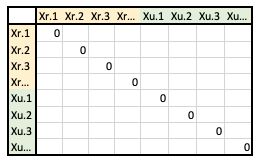
- The matrix format will look like one of the following, depending on how it will be used…
- A. All reference and prediction sets samples as rows and columns (“predictors”)

- B. Reference set samples as rows, prediction set samples as columns (“weights”)

- A. All reference and prediction sets samples as rows and columns (“predictors”)
Neighbor Selection
- The
mbl()function allows you to specify how many nearest neighbors will be used to build local models, by setting eitherk, ork.dissandk.range.- Option 1: Set
kto a sequence of numbers to test, for how many neighbors to include.seq(40, 40, by=20), would perform 1 iteration, using 40 nearest neighborsseq(40, 100, by=20), would perform 4 iterations, using 40, 60, 80 and 100 nearest neighbors
- Option 2:
- Set a dissimilarity threshold
k.dissthat limits the distance to search for neighbors from a sample. You can think of it as the radius of the circles shown in the model theory animation.

- Set
k.rangeto the minimum and maximum number of neighbors you want to include, within thek.dissdistance.
- Set a dissimilarity threshold
- Option 1: Set
Modeling Method
- Once neighbors are selected, MBL builds local models using the multivariate regression method specified with the variable
methodin thembl()function.plsfor partial least squares regressionwapls1for weighted average plsgprfor gaussian process with dot product covariance
pls.callows you to set the number of pls components to be used if either “pls” or “wasp1” is used.- A single number if
plsis used - A vector containing the minimum and maximum number of components to be used, if
wasp1is used
- A single number if
Validation Method
- You can specify the validation method by setting the parameter
valMethodwithin themblControl()function.NNvfor leave-nearest-neighbour-out cross validationloc_crossvalfor local leave group out cross validationnoneIf you chose not to validate the model. This will improve processing speed.
Getting MBL Predictions
MBL predictions are stored in the mbl model as
MODEL$results$model-name$predSince you can run the MBL model with different numbers of nearest neighbors or different dissimilarity thresholds, there can be sets of predictions stored
To choose the best model, we look for the model with the minimum standardized rmse, and extract predictions from this model, using the functions
bestModMBL()andgetPredMBL()sourced fromFunctions/mbl_functions.RIn the demo script,
getPredMBL()is called within a wrapper function,getModResults(). Complete documentation of this function can be found under the Model Performance tab
bestModMBL()
The following function returns the model with the lowest standardized root mean standard error- an index showing how much predictions varied from observations3.
bestModMBL <- function(mbl.sqrt){

  valType <- mbl.sqrt$cntrlParam$valMethod
  if(valType=="NNv"){
    index_best_model <- which.min(mbl.sqrt$nnValStats$st.rmse)
  }
  if(valType=="loc_crossval"){
    index_best_model <- which.min(mbl.sqrt$localCrossValStats$st.rmse)
  }
  best_model_name <- names(mbl.sqrt$results)[index_best_model]

  return(best_model_name)
}
getPredMBL()
This function calls bestModMBL() to choose a model to get predictions from, unless model_name is specified otherwise. Since the lab data was square root transformed when building the model, it is back transformed (squared) after predictions are made.
getLabMBL()
If lab data was input when building the model as Yu, it will be stored at MODEL$results$model-name$yu.obs. Otherwise, you will have to get it from your original prediction dataset